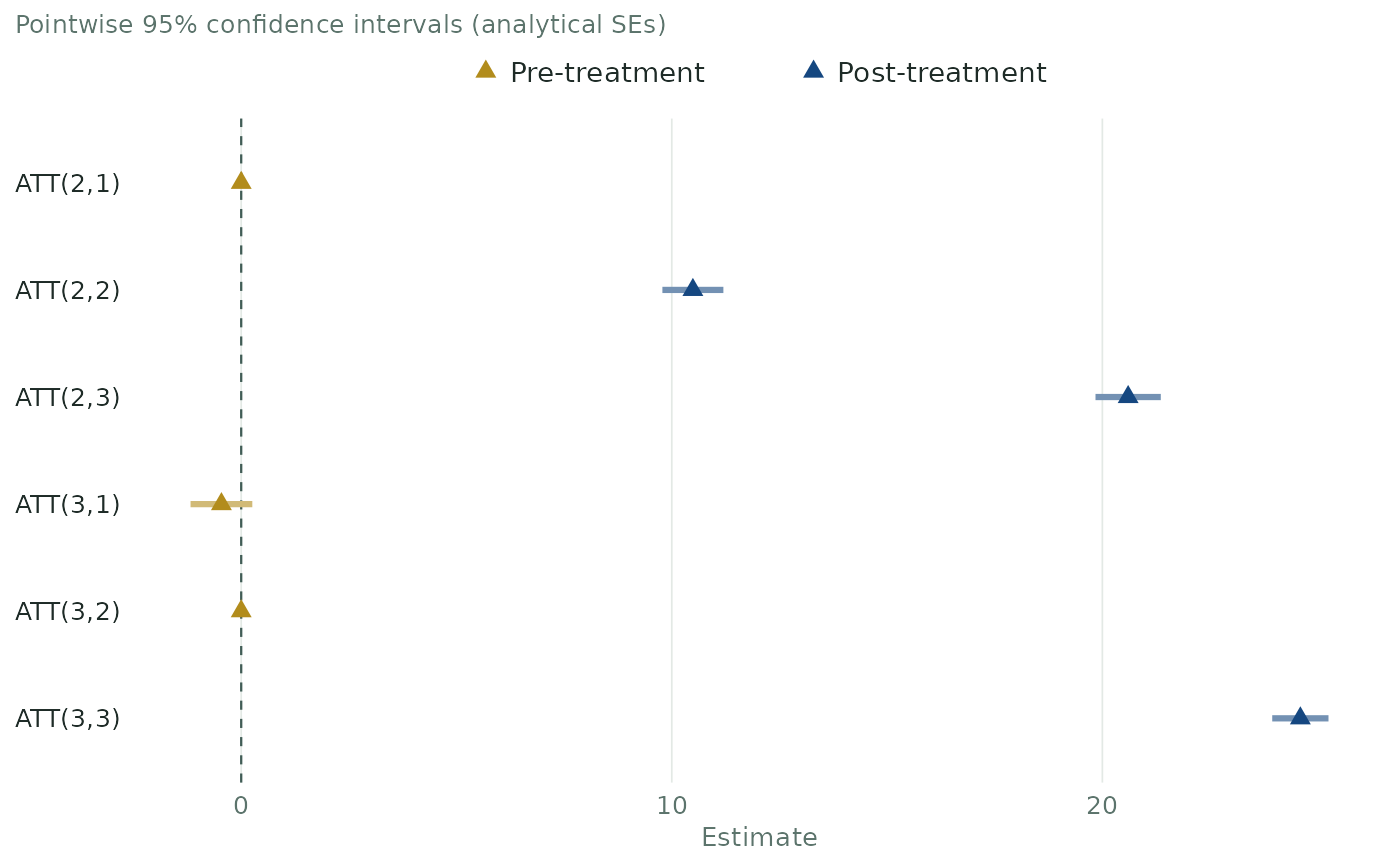
Plot group-time DDD effects
plot.ddd.RdDraws a horizontal coefficient plot of the group-time average treatment
effects ATT(g,t) estimated by ddd(), with one row per ATT(g,t) labelled
"ATT(g,t)". Each estimate is a triangle with its confidence interval as a
thick horizontal bar in a lighter tint of the same color. Pre-treatment
cells (t < g) are gold and post-treatment cells (t >= g) are dark blue.
A dashed vertical line marks zero. For a two-period fit, the plot has a
single row, "ATT".
Usage
# S3 method for class 'ddd'
plot(
  x,
  xlim = NULL,
  xlab = "Estimate",
  ylab = NULL,
  title = NULL,
  subtitle = "auto",
  ...
)
Arguments
- x
A
dddobject returned byddd().- xlim
NULL(default) or a numeric vector of length 2 with finite values. It zooms the horizontal (estimate) axis without removing data. The range shown is always widened to include zero.- xlab
NULLor a single character string for the horizontal axis label. Default is"Estimate".NULLremoves the label.- ylab
NULL(default, no label) or a single character string for the vertical axis label.- title
NULL(default, no title) or a single character string.- subtitle
"auto"(default),NULL, or a single character string."auto"describes the intervals drawn, for example"Pointwise 95% confidence intervals (analytical SEs)".NULLremoves the subtitle.- ...
Not used.
Details
The intervals are the ones stored in the object: the uniform confidence band
when cband = TRUE was used, pointwise intervals otherwise.
The rows keep the order stored in the object (groups in ascending order,
then periods in ascending order), with the first cell at the top. A cell is
pre-treatment when its period is before its group's enabling period
(t < g) and post-treatment otherwise; the legend appears only when both
kinds are present. With a universal base period, the reference cell is
drawn as a point at zero with no interval.
The horizontal axis always includes zero, with or without xlim, so the
zero line is always in view. Estimates that are NA are not drawn, with a
warning.
ggplot2 version 3.5.0 or later must be installed. It is a suggested package.
The result is a regular ggplot object, so it can be changed with +, for
example plot(out) + ggplot2::labs(title = "ATT(g,t)"). A color scale added
with + changes the colors of the triangles and of the bars. To plot an
event study, group or calendar path, aggregate first with agg_ddd() and
plot the result.
Examples
if (requireNamespace("ggplot2", quietly = TRUE)) {
  set.seed(1234)
  data <- gen_dgp_mult_periods(size = 500, dgp_type = 1)[["data"]]
  out <- ddd(yname = "y", tname = "time", idname = "id", gname = "state",
             pname = "partition", xformla = ~cov1 + cov2 + cov3 + cov4,
             data = data, control_group = "nevertreated",
             base_period = "universal", est_method = "dr")
  plot(out)
}